Introduction
Collaborative Filtering (CF) is a strategy used to build recommendation models which are driven by past user behaviour. It can generally be considered in terms of a set of $n$ users who provide feedback on a set of $m$ items. These user interactions can be explicit, like ratings, or implicit like views. The key idea is that each interaction provides some evidence as to the user's preference for the given item.
With this historical preference data, CF approaches can, for example, find similar users based on the item-preferences they have in common, or similar items based on the preferences recorded against them. These associations can then be used to drive recommendations.
Matrix Factorization (MF) is a particular technique for building a CF model, which has been used to great effect when building content recommendation systems. The basic principle of the MF approach is to represent both our users and our items in terms of a set of $f$ shared latent factors, where $f \ll m,n$. In other words, each user is represented by a vector of $f$ numbers and each item is represented by a vector of $f$ numbers. The inner product of these vectors then provides an estimate of the user's preference for the item.
The question we wish to address in this post is: once we have our recommendation model, how do we measure how good it is? In particular, each model has a number of hyperparameters which should to be tuned in order to generate the best model possible. But how do we decide if one model is better or worse than another?
To answer this question we consider a number of established metrics which are used to evaluate classification models, and discuss how they can be applied to the problem at hand.
Building the model
In our previous post we discussed how to build a recommendation system for an implicit feedback dataset by means of Matrix Factorization (MF). That post outlined the theory in pretty fine detail, so we will just recap the relevant results here.
The real beauty of the CF approach is that it is generally applicable and is agnostic to the field of application. The items can be anything: movies, songs, webpages, products in an ecommerce store etc. In our case the items will be learning resources from the GoConqr e-learning platform. The interactions which we consider are the number of times that each user has viewed each resource. Because the user has not explicitly stated their approval for the resource this is considered to be implicit feedback. In particular, the fact that a user has not viewed a resource should not be interpreted as a strong signal that the user disapproves of the resource; this fact will be very relevant later.
The structure of the raw data can be seen from the short extract below, which is comprised of three columns: user_id (anonymized), resource_id
and number_of_views:
adddaf35-9f11-46c5-a73b-ce1877c98af6,489473,1
adddaf35-9f11-46c5-a73b-ce1877c98af6,497329,1
9ad79045-984b-42c0-819f-6433f037189b,608278,1
f2d4beb2-01b2-4173-8526-ec2a8020321f,722458,2
f2d4beb2-01b2-4173-8526-ec2a8020321f,1751655,1
f2d4beb2-01b2-4173-8526-ec2a8020321f,2811071,1
2e4678f9-941f-4a7a-9509-f4e64a49fad9,155869,1
2e4678f9-941f-4a7a-9509-f4e64a49fad9,1958564,1
2e4678f9-941f-4a7a-9509-f4e64a49fad9,18559518,8
2e4678f9-941f-4a7a-9509-f4e64a49fad9,19722753,1
2e4678f9-941f-4a7a-9509-f4e64a49fad9,21019720,2
0a5ca2dd-9fe9-4de4-9fa3-8900a43a69fb,146521,1
0a5ca2dd-9fe9-4de4-9fa3-8900a43a69fb,296809,1
We load this data into a $n \times m$ matrix, $R$. Each distinct user will be represented by a row in $R$, with the elements in the row representing the number of times the user viewed each resource. As a consequence, each column in $R$ can be considered to represent a single resource, with the elements in the column representing how many views the resources received from each user: $$ R = \left( \begin{array}{cccc} r_{1,1} & r_{1,2} & \cdots & r_{1,m} \\ r_{2,1} & r_{2,2} & \cdots & r_{2,m} \\ \vdots & \vdots & \ddots & \vdots \\ r_{n,1} & r_{n,2} & \cdots & r_{n,m} \end{array} \right) \tag{1}\label{1}, $$
Separating training and test data
Before training our model we need to split off some data which will remain unseen during training, and which can be used to later evaluate our
model. In the previous post we listed the make_train function (see [2]), and we
reproduce it again here for convenience:
import random
import numpy as np

def make_train(ratings, percentage_test = 0.2):
    '''
   Takes original ratings matrix in CSR format and returns a training set, a test set and a list of of the user_ids with
    omissions in the training set.
    '''
    test_set = ratings.copy() # Make a copy of the original set to be the test set.
    test_set[test_set != 0] = 1 # Store the test set as a binary preference matrix
    training_set = ratings.copy() # Make a copy of the original data we can alter as our training set.
    nonzero_inds = training_set.nonzero() # Find the indices in the ratings data where an interaction exists
    nonzero_pairs = list(zip(nonzero_inds[0], nonzero_inds[1])) # Zip these pairs together of user,item index into list
    random.seed(0) # Set the random seed to zero for reproducibility
    num_samples = int(np.ceil(percentage_test*len(nonzero_pairs))) # Round the number of samples needed to the nearest integer
    samples = random.sample(nonzero_pairs, num_samples) # Sample a random number of user-item pairs without replacement
    user_inds = [index[0] for index in samples] # Get the user row indices
    item_inds = [index[1] for index in samples] # Get the item column indices
    training_set[user_inds, item_inds] = 0 # Assign all of the randomly chosen user-item pairs to zero
    training_set.eliminate_zeros() # Get rid of zeros in sparse array storage after update to save space
    return training_set, test_set, list(set(user_inds)) # Output the unique list of user rows that were altered
This method takes the full dataset, ratings, and makes two copies of the data, test_set and training_set.
The test_set is cast into a binary format; it no longer reflects the number of views the user has registered against each resource, but
simply indicates if there has been an interaction. When we evaluate our model at the end, we will be comparing against this binarized format.
We then find the indexes of all the non-zero views in the ratings data, and we take a random sample of these non-zero interactions (20% by default).
For this sample of interactions the training_set is altered to equal zero, removing the interaction. The method then returns the
training and test sets, along with an array indicating the particular user rows for which interactions had been removed.
The basic idea is that we train our model with a training_set that excludes some known interactions. Then, once we have our model, we
want to see how well the model will be able to recreate these non-zero interactions which had been removed from the training data.
Building the MF model
The Matrix Factorization approach attempts to decompose our large $n \times m$ matrix, $R$ $\eqref{1}$, into a product of two separate matrices: $$ \begin{aligned} R &= X^{\rm{T}}.Y \\ &=\left( \begin{array}{cccc} x_{1}^{1} & x_{1}^{2} & \cdots & x_{1}^{f} \\ x_{2}^{1} & x_{2}^{2} & \cdots & x_{2}^{f} \\ \vdots & \vdots & \ddots & \vdots \\ x_{n}^{1} & x_{n}^{2} & \cdots & x_{n}^{f} \end{array} \right) \times \left( \begin{array}{cccc} y_{1}^{1} & y_{2}^{1} & \cdots & y_{m}^{1} \\ y{1}^{2} & y_{2}^{2} & \cdots & y_{m}^{2} \\ \vdots & \vdots & \ddots & \vdots \\ y_{1}^{f} & y_{2}^{f} & \cdots & y_{m}^{f} \end{array} \right) \tag{2}\label{2} \end{aligned} $$
Here we have introduced the $f \times n$ matrix, $X$, and the $f \times m$ matrix, $Y$. The column $u$ of matrix $X$ is a vector describing the user $u$ in terms of $f$ latent factors, and we will henceforth refer to this as $\mathbf{x}_{u}$.
On the other side, the matrix $Y$ may also be considered to be made up of column vectors of length $f$. In this case the column vector $i$ is a description of item $i$, which we will denote as $\mathbf{y}_{i}$. We try to describe our items in terms of the same $f$ factors that we use to describe our users.
The task in Matrix Factorization is to find the elements of the matrices $X$ and $Y$ which reconstruct $R$ most accurately. If we take a look at $\eqref{2}$ we see that once we have calculated our user and item matrices, $X$ and $Y$, we should be able to reconstruct any element of $R$ ($r_{ui}$) by taking the inner product of the user vector $\mathbf{x}_{u}$ with the item vector $\mathbf{y}_{i}$: $$ \hat{r}_{ui} = \mathbf{x}_{u}^{\rm{T}}.\mathbf{y}_{i} = \sum_{j=1}^{f} x_{u}^{j}.y_{i}^{j} \tag{3}\label{3} $$
We use optimization techniques (see [1]) to determine the elements of matrices $X$ and $Y$ which will recreate the $r_{ui}$ in our training data most accurately. Once we have our matrices $X$ and $Y$ we have our model. We can then use these matrices to estimate the preference of any user for any item, according to $\eqref{3}$.
Comparing our model to test data
To evaluate the model we need to compare the predicted interactions, $\hat{r}_{ui}$ from $\eqref{3}$, with unseen interactions in our test set. We introduce the
CFEvaluator class to carry out this task. It will need to be instantiated with the model we have just trained, the training data, the test data
and the list of user IDs that were altered before training:
from sklearn import metrics
import numpy as np

class CFEvaluator(object):
    def __init__(self, model, train_data, test_data, user_idxs_altered):
        self.model = model
        self.train_data = train_data
        self.test_data = test_data
        self.user_idxs_altered = user_idxs_altered
        …
The class will expose a method, mean_metric, for calculating different evaluation metrics for the model. The method is called
mean_metric because we will follow the pattern of evaluating the metric for each example user, then take the average value
across all of these example users. What do I mean by an example user? These are just the known users for whom the traning data had been
amended to remove existing inteactions, i.e. user_idxs_altered.
    def mean_metric(self, metric="auc"):
        model_metric = [] # Empty list to store model evaluations for each user
        popularity_metric = [] # Empty list to popularity based evaluations for each user
        pop_items = np.array(self.test_data.sum(axis = 0)).reshape(-1) # Get sum of item iteractions to find most popular
        item_vecs = self.model.embeddings()["items"] # Latent factor representation of our items
        for user_idx in self.user_idxs_altered: # Iterate through each user that had an item altered
            training_row = self.train_data[user_idx,:].toarray().reshape(-1) # Get the training set row
            zero_inds = np.where(training_row == 0) # Find where the interaction had not yet occurred in training data

            # Get the predicted values based on our user/item vectors
            user_vec = self.model.embeddings()["users"][user_idx,:]
            pred = user_vec.dot(item_vecs.T)[zero_inds].reshape(-1)

            # Get corresponding binarized interactions from the test data
            actual = self.test_data[user_idx,:].toarray()[0,zero_inds].reshape(-1)
            pop = pop_items[zero_inds] # Get the item popularity for our chosen items
            if metric=="auc":
                model_metric.append(self._auc_score(pred, actual))
                popularity_metric.append(self._auc_score(pop, actual))
           …
            # End users iteration

        # Return mean of the evaluation metric for our CF model and the popularity benchmark
        return float('%.3f'%np.mean(model_metric)), float('%.3f'%np.mean(popularity_metric))

        …

   def _auc_score(self, predictions, test):
       return metrics.roc_auc_score(test, predictions)
This method will loop over each of the example users and will calculate and store the evaluation metric for that user. It will also calculate and store the same metric for a simple popularity-based model. Once this has been done for each of the altered users, the average value for the metric is returned for both the CF model being assessed and the popularity-based model. To calculate the metric for each example user we do the following:
- Extract the training data for the user and find all items for which no interactions had been recorded in the training data; we will filter our predictions and test data to only consider those resources for which the user did not register an interaction in the training data, i.e. we exclude the red columns in Fig 1.
- Generate our model predictions by multiplying the user vector, in latent factor space, against each of the items. Filter these predictions to the subset of 'non-interacted' resources identified above.
- Extract the corresponding binarized preference data from the test set by, again, filtering on the 'non-interacted resources' identified from the training set.
-
Pass the prediction array and the test (or actual) array to the the metric calculator. In the following section we will discuss the different evaluation metrics, to better
understand how each of them will be calculated. In most cases we will use existing
scikitlearnimplementations to calculate the metrics, but understanding what these metrics are representing is key to choosing the correct one.
| Resource index | 0 | 1 | 2 | 3 | 4 | 5 | 6 | 7 | 8 | 9 |
|---|---|---|---|---|---|---|---|---|---|---|
| Raw data | 0 | 2 | 0 | 0 | 1 | 3 | 0 | 0 | 8 | 0 |
| Training | 0 | 0 | 0 | 0 | 1 | 0 | 0 | 0 | 8 | 0 |
| Test data | 0 | 1 | 0 | 0 | 1 | 1 | 0 | 0 | 1 | 0 |
| Predictions | 0.1 | 0.6 | 0.05 | 0.02 | 0.8 | 0.45 | 0.2 | 0.01 | 0.77 | 0.73 |
Notice how our raw data shows how many interactions (or views) are recorded against each of the resources, $0-9$. To create our training row we randomly zero some of the columns for which interactions were seen (columns 1 and 5 in this case). The test set is just a binarized representation of the the original (raw) data. The predictions row is the output of our model, giving some relative measure of the precited interations between the user and each of the resources, $0-9$. The first step in evaluating our model is to strip out the red columns (4 and 8) where we know, from our training data, that a positive interaction has occurred.
Confusion matrix
The starting point for each metric is a pair of equal-length arrays pertaining to a single user. One array (predictions) represents the predictions made
by our model; elements in the array estimating the user's preference for each resource. The other array, test, is a binary representation of whether or not the user has
interacted with the resource. We want to evaluate how closely our predictions array matches the actual test data. To illustrate, let's consider the dummy data which was presented
in Fig 1. The original 10 elements have now been filtered down to 8, as we have removed the resources for which the training data already contained an interaction, i.e. indicies 4 and 8.
The comparison of our predictions to our test data can be seen in Fig 2., where the green shaded columns representdoesn't resources where the test
data has indicated an historical interaction.
| Resource index | 0 | 1 | 2 | 3 | 5 | 6 | 7 | 9 |
|---|---|---|---|---|---|---|---|---|
| Test data | 0 | 1 | 0 | 0 | 1 | 0 | 0 | 0 |
| Predictions | 0.1 | 0.6 | 0.05 | 0.02 | 0.45 | 0.2 | 0.01 | 0.73 |
To make use of established evaluation metrics it is convenient to treat our model as a binary classifier; for this, our model should assign, to each resource, a value of $1$, to indicate an appropriate recommendation or a $0$ otherwise. Thus, we need to translate our predictions, which take the form of probabilities or scores, into binary indicators. We can achieve that by applying a threshold, where probabilities above this threshold will be assigned $1$ and values below, $0$. Let's apply a threshold of 0.5 to our current predictions:
| Resource index | 0 | 1 | 2 | 3 | 5 | 6 | 7 | 9 |
|---|---|---|---|---|---|---|---|---|
| Test data | 0 | 1 | 0 | 0 | 1 | 0 | 0 | 0 |
| Predictions (threshold 0.5) | 0 | 1 | 0 | 0 | 0 | 0 | 0 | 1 |
Comparing our binarized predictions to the test data we can see a number of different categories which are common for any binary classified and are encoded in the
confusion matrix:
Predicted 0 Predicted 1
Actual 0 TN: 0, 3, 2, 6, 7 FP: 9
Actual 1 FN: 5 TP: 1
- True positive ($TP$): Predictions indicate an appropriate recommendation and test data reveals an interaction was measured (resource 1)
- True negative ($TN$): Predictions do not indicate an appropriate recommendation and test data reveals that, indeed, no interaction was measured (resources 0, 3, 2, 6 and 7)
- False negative ($FN$): Predictions do not indicate an appropriate recommendation but test data reveals that an interaction was measured (resource 5)
- False positive ($FP$): Predictions indicate an appropriate recommendation but test data reveals that no interaction was measured (resource 9)
The key complication with this implicit feedback recommender is that we can't really identify false positives. The fact that the user did not register an historical preference for an item does not mean that they disapprove of the item, they may simply have not been exposed to it. In fact, identifying and recommending items where the user has not had an historical interaction is exactly the purpose of the recommender. In our example above, resource 9 is classified as a false positive but it is clearly the resource that our model would recommend for this user.
This problem with identifying false positives for implicit feedback data will ultimately dictate the evaluation metric that we use to evaluate our model.
Precision and recall
Building on the definitions introduced for our confusion matrix we meet the metrics precision and recall. Precision measures the proportion of true positives to the total number of positives predicted by our model: $$ \rm{precision} = \frac{TP}{TP + FP} \tag{4}\label{4} $$ We can improve the precision of our model by only predicting positive cases where we are very confident in the prediciton, i.e. increasing our threshold. This strategy will increase the chances for us to miss some positive cases, but it will reduce the number of false postives and thereby increase precision. But failing to identify some positive cases is also undesirable and this is what is captured by the recall metric (or true positive rate), which compares the number of true positives that our model identifies against the total number of actual positives in the test data $$ \rm{recall} = TPR =\frac{TP}{TP + FN} \tag{5}\label{5} $$ We can increase the recall of our model by reducing the threshold for positive classification, but this will have the corollary effect of decreasing precision. In fact, we can always, trivially, achieve a recall of 1 by simple setting our threshold low enough to return all cases. The behaviour or our binary classifier model can be characterised by the precision-recall (PR) curve, where the values of precision and recall are plotted for different threshold values. Below we plot the PR curve as generated for our recommendation model running against a single user.
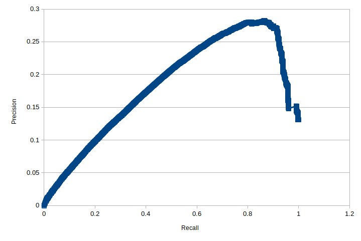
The curve in Fig 5a is a long way from our textbook precision-recall curve, which looks something more like this:
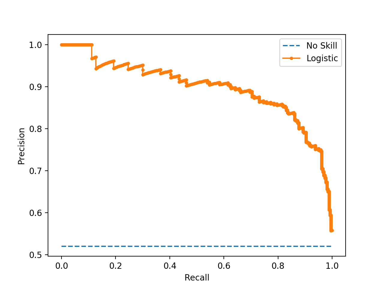
However, the plot for our CF model in Fig 5a. does not demonstrate these expected features. We see that the recall does indeed achieve a value of 1 at a low threshold. As the threshold increases the recall will drop and the precision initially increases as we would expect, but as the recall drops below 0.85 the precision also starts to drop. What gives?
The problem with our PR curve is again rooted in our inability to correctly identify the false positive cases. If we consider our dummy data once more from Fig 2., and consider what will happen if we now apply a threshold of 0.7:
| Resource index | 0 | 1 | 2 | 3 | 5 | 6 | 7 | 9 |
|---|---|---|---|---|---|---|---|---|
| Test data | 0 | 1 | 0 | 0 | 1 | 0 | 0 | 0 |
| Predictions (threshold 0.7) | 0 | 0 | 0 | 0 | 0 | 0 | 0 | 1 |
In this case our model only makes a single positive prediction for index 9, which has no interaction reflected in our test data and so must be classified as a false postitive. Evaluating the precision for this case gives $\frac{TP}{TP +FP}=0$, increasing the threshold has actually caused a reduction in our precision. So we see that the precision metric, and the precision-recall curve, appear inappropriate for our implicit feedback data. Perhaps we can have more confidence in the ROC curve.
ROC Curve
A very similar analysis can be done with the receiver operating characteristic (ROC) curve. Thhe ROC curve plots the true positive rate, which is identical to the recall, against the false positive rate, which is defined as: $$ \rm{FPR} = \frac{FP}{TN + FP} \tag{6}\label{6} $$ As for the PR curve, we can plot this ROC curve for a sample user:
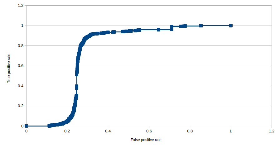
Again the position of the elbow in the plot is the important charateristic, the futher this is pushed into the top-left corner the better is your classifier. And once again the area under the curve is the appropriate metric to enumerate this, with values approaching 1 being better and values approaching 0.5 representing a random classifier. In this case the curve is a bit closer to our textbook examples, so lets use this ROC plot to evaluate our model and optimize for the hyperparameter $f$, i.e. the number of latent factors which we use to represent our users and items. Below we look at the model generated for different $f$ and for each case we evaluate the area under the ROC curve
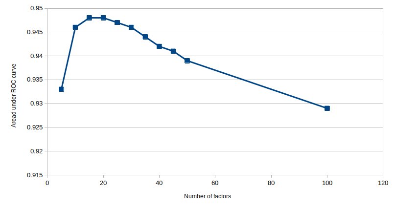
The plot demonstrates a clear maximum around $f=20$, suggesting that our optimal representation in this case should contain 20 latent factors.
Mean Percentage Ranking
The problem with both the PR and ROC curve, in our case, is that they both rely on being able to enumerate the number of false positives; notice the dependence of $FP$ in both $\eqref{4}$ and $\eqref{6}$. But as we have noted on a couple of occasions, our implicit feedback does not contain any negative feedback which makes it difficult or impossible to correctly identify false positives. To address this we can use a recall-based metric known as the mean percentage rank (MPR), see ref [4]. To calculate this metric we use our predictions for user, $u$, to rank each of the resources, $i$, from our best recommendation down to our worst. We then assign a percentage rank, $rank_{ui}$, for all the items in the list, such that the top-most item will be 0% and the last item 100%. The mean-percentage rank is then given by $$ MPR = \frac{\sum_{u,i} r_{ui} rank_{ui}}{\sum_{u,i} r_{ui}} $$ We can apply this formula to our dummy example from earlier to better understand how this calculation is arrived at in the case of a single user. We sart with the data presented in Fig 2, but with the predictions placed in rank order, notice the re-ordering in the resource indices:
| Resource index | 9 | 1 | 4 | 5 | 0 | 2 | 3 | 7 | $\sum_{i}$ |
|---|---|---|---|---|---|---|---|---|---|
| Predictions | 0.73 | 0.6 | 0.45 | 0.2 | 0.1 | 0.05 | 0.02 | 0.01 | |
| % Rank, $rank_{ui}$ | 0 | 14.29 | 28.57 | 42.85 | 57.14 | 71.43 | 85.71 | 100 | |
| Test data, $r_{ui}$ | 0 | 1 | 1 | 0 | 0 | 0 | 0 | 0 | 2 |
| $r_{ui}.rank_{ui}$ | 0 | 14.29 | 28.57 | 0 | 0 | 0 | 0 | 0 | 42.85 |
We see that for this particular dummy user the MPR evaluates to $\frac{42.85}{2}=21.43$. We have only calulated the metric for a single user here, the actual metric is calculated over all $u$ and $i$, but the interpretation is the same. If you have a low value for $MPR$ (< 50%) that means that more of actual user interactions have occurred for the items at the top of our ranked list, which is a good sign. If more actual interactions are observed for the items at the bottom of our ranked list the value for MPR will increase. If our recommendations were completely random we would expect MPR to evaluate to about 50%.
The implementation for this metric is shown below, in the context of our CFEvaluator class introduced above:
class CFEvaluator(object):
    …
    def mean_percentage_rank(self):
        sum_weighted_ranks = 0
        sum_weighted_ranks_pop = 0
        sum_total_actual = 0

        pop_items = np.array(self.test_data.sum(axis = 0)).reshape(-1) # Get sum of item iteractions to find most popular
        item_vecs = self.model.embeddings()["items"] # Latent factor representation of our items
        for user_idx in self.user_idxs_altered: # Iterate through each user that had an item altered
            training_row = self.train_data[user_idx,:].toarray().reshape(-1) # Get the training set row
            zero_inds = np.where(training_row == 0) # Find where the interaction had not yet occurred in training data

            # Get the predicted values based on our user/item vectors
            user_vec = self.model.embeddings()["users"][user_idx,:]
            predictions = user_vec.dot(item_vecs.T)[zero_inds].reshape(-1)

            # Get corresponding binarized interactions from the test data
            actual = self.test_data[user_idx,:].toarray()[0,zero_inds].reshape(-1)
            popular = pop_items[zero_inds]

            # Keep running summation of numerator and demoninator for MPR
            sum_weighted_ranks += self._sum_weighted_rank(predictions, actual)
            sum_weighted_ranks_pop += self._sum_weighted_rank(popular, actual)
            sum_total_actual += sum(actual)

        return float('%.3f'%(sum_weighted_ranks/sum_total_actual)), float('%.3f'%(sum_weighted_ranks_pop/sum_total_actual))

    def _sum_weighted_rank(self, predictions, test):
        n = len(predictions)
        ranked = sorted(zip(predictions, test), key=lambda el: el[0], reverse=True)
        return sum([ 100*pred[1]*count/n for count, pred in enumerate(ranked) ])
Let's look at how this MPR value changes as we vary the interaction weight, $\alpha$, which is a hyperparameter of our model
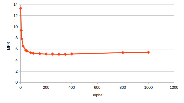
There is a minimum in this plot around $\alpha=250$, which is illustrated more clearly when we consider the $\log_{10}\left( \alpha \right)$:
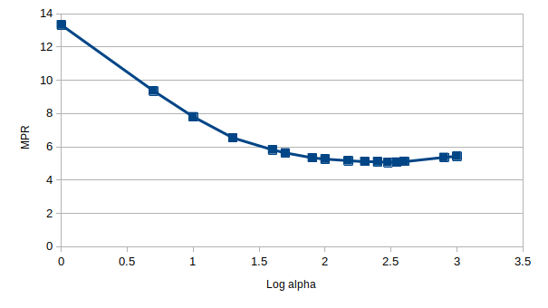
Beautiful. We see tha the MPR provides a much more meaningful metric for us to evaluate our implicit feedback model, by virture of the fact that it is not as sensitive to false-positive classifications. However, it should be noted that the calculation presented here is a good deal slower than the alternative evaluation metrics presented, i.e. area under the PR and ROC curves.
Conclusion
In this post we have taken a deep dive into the evaluation of the collaborative filtering model trained in our previous post. To evaluate this model we framed it as a binary classifier which classified resources as being either appropriate or not appropriate to the target user. Prior to training, our raw data was separated into training and test sets; the training set had a random selection of user-item interactions removed. To evaluate the model we compared our predictions to the full dataset, excluding any interactions we already know from the training set.
We introduced a number of evaluation metrics, and explained how these could be calculated for the present model, including the confusion matrix, precision, recall and area under the ROC curve. We explained that all of these metrics shared the short-coming that we could not reliably determine the false positives for our implicit feedback data, which led us to consider the more appropriate metric of Mean Percentage Rank. We showed how this metic is implemented and examined how the metric varies for the current recommendation model, demonstrating the optimization of selected hyperparameters of the model.
References
- Seminal paper on collaborative filtering for implicit feedback datasets from Hu, Koren & Volinsky
- Great Python Notebook from Jesse Steinweg-Woods demonstrating the ALS method for implicit data
- The implicit library from Ben Frederickson
- Logistic matrix factorization by Christopher Johnson from which we take the MPR evaluation metric
- Machine Learning Mastery article about precsion-recall curves
Comments
There are no existing comments
Got your own view or feedback? Share it with us below …