Introduction
GoConqr is a free e-learning platform that provides a set of tools for creating and sharing learning content, including mindmaps, flashcards, quizzes, slides, notes and flowcharts. Over the years it has accumulated a vast public library of user-generated content, across all imaginable topics, from users around the globe.
A lot of the content created is throw-away and not of much use to other learners, but some of the content is of exceptionally high quality and provides benefit far beyond the boundaries of its original intended audience.
At GoConqr we want to surface this high-quality content to the users who could benefit from it, however, we often possess limited meta information about the content. We are lucky if the author bestows their work with a title and a description, and much less likely for the author to aid our classification of the content with information like subject, topic, learning level or other tags. We have used this meta data, where it exists, to drive recommendations, but this approach has its limitations.
One piece of data that we do hold about these learning resources is which logged-in users have viewed them, and how frequently. With this data we can consider the use of collaborative-filtering approaches to make resource recommendations. In this post I will describe the technique of collaborative filtering and I will show how we can apply these techniques to a data extract from GoConqr, enabling us to build a resource recommendation system.
Recap on the Theory of Collaborative Filtering
There are a number of different approaches you can use to build a recommendation system. In one approach we can attempt to represent our users and resources by means of a set of concrete features which we collect. For the GoConqr e-learning example we could describe our users in terms of their age, their country, their language, their level of study, the subjects they study etc. In a similar way, the learning content could be described by the level of study to which it is appropriate, when it was created, the subject it relates to, and the specific topic within that subject etc. Describing our content in this way can allow us to map users who share a particular set of criteria over to a set of learning resources which will (presumably) be of interest to them. One of the major drawbacks of this approach is that we need to collect all of these data points about our users and the learning resources. Collection of this type of meta-data is both onerous and error-prone.
The technique of Collaborative Filtering (CF) offers an interesting alternative. Instead of worrying about these concrete features of the users and learning resources we can instead just look at historical user preferences for different resources. The prototypical CF example will consider users' ratings for different movies (e.g. on a 5-star scale or a thumbs-up/thumbs-down), and it will then make suggestions for a given user based on their rating history. The recommendations will be built from the preferences of other users who have shown similar historical preferences to the target user.
Matrix Factorization (MF) is one approach to collaborative filtering that has proven very successful across a wide range of applications. This approach came to prominence after the ideas were published by Simon Funk whilst working towards the Netflix prize in 2006. In this approach we consider that the original user ratings can be represented as an $n \times m$ matrix, $R$: $$ R = \left( \begin{array}{cccc} r_{1,1} & r_{1,2} & \cdots & r_{1,m} \\ r_{2,1} & r_{2,2} & \cdots & r_{2,m} \\ \vdots & \vdots & \ddots & \vdots \\ r_{n,1} & r_{n,2} & \cdots & r_{n,m} \end{array} \right) \tag{1}\label{1}, $$
where $n$ is the number of users, $m$ is the number of resources and $r_{u,i}$ is the rating given by user $u$ to item $i$.
In this representation you can consider any row $u$ of the matrix $R$ to be feature vector representing the user $u$. The $m$-dimensional vector is comprised of the ratings that user $u$ has bestowed upon each of the $m$ items.
Similarly any column $i$ of the matrix $R$ can be considered to be a feature vector representing the item $i$, comprised of all the ratings assigned to that item by the $n$ users.
It is worth noting, at this point, that this matrix, $R$ can get very large, even for modestly sized systems. For example, the GoConqr dataset we consider here could easily end up encompassing >100K users and 10K different resources, which will mean matrix $R$ will have over 1 billion elements.
Where the user has provided a rating for the item this rating will populate the corresponding element, $r_{u,i}$. However, for most of the cases we will not have an existing rating. The goal of the recommender system is to provide some way to fill-in the missing elements of the matrix, where an interaction (or rating) has not yet been registered. We will denote our guess for the missing value by $\hat{r}_{u,i}$, and our recommendations will be based on where the values of $\hat{r}_{u,i}$ are largest.
The Matrix Factorization approach attempts to decompose this single, large $n \times m$ matrix, into a product of two separate matrices: $$ \begin{aligned} R &= X^{\rm{T}}.Y \\ &=\left( \begin{array}{cccc} x_{1}^{1} & x_{1}^{2} & \cdots & x_{1}^{f} \\ x_{2}^{1} & x_{2}^{2} & \cdots & x_{2}^{f} \\ \vdots & \vdots & \ddots & \vdots \\ x_{n}^{1} & x_{n}^{2} & \cdots & x_{n}^{f} \end{array} \right) \times \left( \begin{array}{cccc} y_{1}^{1} & y_{2}^{1} & \cdots & y_{m}^{1} \\ y{1}^{2} & y_{2}^{2} & \cdots & y_{m}^{2} \\ \vdots & \vdots & \ddots & \vdots \\ y_{1}^{f} & y_{2}^{f} & \cdots & y_{m}^{f} \end{array} \right) \tag{2}\label{2} \end{aligned} $$
Here we have introduced the $f \times n$ matrix, $X$, and the $f \times m$ matrix, $Y$. The column $u$ of matrix $X$ is a user vector that describes user $u$, and we will henceforth refer to this as $\mathbf{x}_{u}$. This vector is of length $f$, and the model is essentially trying to describe the user $u$ by means of $f$ separate numbers, these $f$ dimensions are termed the features or factors of the model.
On the other side the matrix $Y$ may also be considered to be made up of column vectors of length $f$. In this case the column vector $i$ is a description of item $i$, which we will denote as $\mathbf{y}_{i}$. We try to describe our items in terms of the same $f$ factors that we use to describe our users.
The use of these common factors to describe our users and items is analagous to our simple recommendation model described at the outset. In this earlier example we classified users by their concrete features like subject and level of study. We then tried to match these users to resources which have similar categorization for subject and level of study. In both cases we are looking for a strong overlap between the features describing the users and those describing the resources, however, in the case of matrix factorization the $f$ features we use to describe our users/items are more abstract. The method of factorization selects these factors and their values, not on the basis of their concrete physical meaning, but rather because they are simply the numbers which give us the best average predictions; they are often referred to as latent factors. But what are the predictions of this MF model?
The task in Matrix Factorization is to find the elements of the matrices $X$ and $Y$ which reconstruct $R$ most accurately. If we take a look at $\eqref{2}$ we should be able to deduce that once we have calculated our user and item matrices, $X$ and $Y$, we can reconstruct any element of $R$ ($r_{u,i}$) by taking the inner product of the user vector $\mathbf{x}_{u}$ with the item vector $\mathbf{y}_{i}$: $$ \begin{aligned} \hat{r}_{u,i} &= \mathbf{x}_{u}^{\rm{T}}.\mathbf{y}_{i} \\ &= \sum_{j=1}^{f} x_{u}^{j}.y_{i}^{j} \tag{3}\label{3} \end{aligned} $$
This inner product of the user and item vectors determines the overlap of the shared factors describing the user, $u$, and the item $i$, and this provides our prediction for $r_{u,i}$. If we consider that our goal with this factorization is to minimize the difference between our predicted interactions ($\hat{r}_{u,i}$) and the actual measured interactions ($r_{u,i}$) we can see that the matrix factorization can be phrased as an optimization problem where we aim to minimize the following cost/loss function: $$ \begin{aligned} \sum_{ {u,i} } \left( r_{u,i} - \hat{r}_{u,i} \right)^{2} + \lambda_{x} \sum_{u=1}^{f} \left\lVert \mathbf{x}_{u} \right\rVert + \lambda_{y} \sum_{i=1}^{f} \left\lVert \mathbf{y}_{i} \right\rVert \\ =\sum_{ {u,i} } \left( r_{u,i} - \mathbf{x}^{T}_{u} . \mathbf{y}_{i} \right)^{2} + \lambda_{x} \sum_{u=1}^{n} \left\lVert \mathbf{x}_{u} \right\rVert + \lambda_{y} \sum_{i=1}^{m} \left\lVert \mathbf{y}_{i} \right\rVert \end{aligned} $$
The first summation is over all of the combinations of ${u, i}$ for which we have actual interaction or rating data. This summation finds the total squared error in the preductions made by our model compared to the actual rating data.
As well as minimizing the mean-squared-error of our predictions, this cost function also adds regularization through the Lagrange multipliers, $\lambda_{x}$ and $\lambda_{y}$. This regularization aims to apply a pressure, during the optimization process, which should encourage the user and item factors to take smaller values, closer to zero; this should prevent the factors from overfitting the data used during training and help our final model to generalize better. These hyperparameters should be optimized using cross validation on our data. Often we will settle on tuning a single regularization parameter: $$ \begin{aligned} \sum_{ {u,i} } \left( r_{u,i} - \mathbf{x}^{T}_{u} . \mathbf{y}_{i} \right)^{2} + \lambda \left( \sum_{u=1}^{n} \left\lVert \mathbf{x}_{u} \right\rVert + \sum_{i=1}^{m} \left\lVert \mathbf{y}_{i} \right\rVert \right) \tag{4}\label{4} \end{aligned} $$
But before we get to the calculation of our model we have one significant extension to discuss.
Matrix factorization for implicit feedback datasets
Using matrix factorization in the way defined relies on having suffient real user ratings, $r_{u,i}$, to build a robust model. The summation in the loss function only encompasses the combinations of ${u,i}$ where we have a rating. This technique runs into problems when we have a highly sparse dataset with very little interaction. In the case of the GoConqr dataset, we are considering the number of times each user has viewed each resource, and a given user will only have viewed a tiny proportion of all of the (~10K) available resources. But what can we say when a user hasn't viewed a resource? Is the user not interested in the resource? Possibly, or perhaps the user has not yet encountered the resource. Similarly, just because a user has viewed a resource does not mean that they have liked it; it's a positive indication but it is a long way from an endorsement. However, what if the user has viewed the same resource 10 times? That would certainly seem to be a strong indication that they found the resource useful. Hopefully you can get an idea of where we are going with this: when we are considering implicit datasets we have no certainty of the user's preference, we make statements with a variable level of confidence.
The model for implicit data requires that we introduce the binarized user preference, $p_{u,i}$, where: $$ p_{u,i} = \begin{cases} 1 & r_{u,i} > 0 \\ 0 & r_{u,i} = 0 \end{cases} $$
We also introduce the confidence we have in each $p_{u,i}$, and this is represented by $c_{u,i}$. When the user has not registered any views against the resource we will assert that the user has no preference, i.e. $p_{u,i}=0$. However our confidence in this statement will be small (i.e. 1), for the reasons discussed above. Once the user registers any view against a resource we will assert that a preference now exists and $p_{u,i}=1$. With a small number of views our confidence in this assertion will be small but it should grow as the user registers more views against the resource. We can capture these ideas with a simple linear relationship between $c_{u,i }$ and $r_{u,i}$, for example: $$ c_{u,i} = 1 + \alpha r_{u,i} , $$
where $\alpha$ is a hyperparameter for the model, and can be found by experimentation. We can then rephrase our previous cost function in terms of our new $p_{u,i}$ and $c_{u,i}$ variables: $$ \begin{aligned} \sum_{u=1}^{n} \sum_{i=1}^{m} c_{u,i}\left( p_{u,i} - \mathbf{x}^{T}_{u} . \mathbf{y}_{i} \right)^{2} + \lambda \left( \sum_{u=1}^{n} \left\lVert \mathbf{x}_{u} \right\rVert + \sum_{i=1}^{m} \left\lVert \mathbf{y}_{i} \right\rVert \right) \tag{5}\label{5} \end{aligned} $$
Notice the fundamental difference from the cost function $\eqref{4}$, we now have a term for every user ($u$) and item ($i$) combination. For the previous explicit feedback cost function we only considered where the user had provided a rating, i.e. where $r_{u,i}$ existed. We now have a term for each combination because the $c_{u,i}$ will always have some non-zero value, which is just very small in the case where ther has been no interaction. Our error function will also factor in how well our latent factor representation, $\mathbf{x}^{T}_{u} . \mathbf{y}_{i}$, predicts the case where there has been no interaction. In other words, if we see no interaction we expect our latent factor representation to also reflect that, but our low $c_{ui}$ means that we are quite tolerant of error in these cases.
With our cost function defined, our task is to determine the elements of the user vectors, $\mathbf{x}_u$, and the resource vectors, $\mathbf{y}_{i}$ as seen in $\eqref{3}$. And the values of these vectors should be selected such that they minimize the cost function in equation $\eqref{5}$.
For further discussion on how one can solve this optimization problem efficiently the reader is directed to the original paper [1]. For our purposes we will use the implementation of this algorithm provided in the implicit library. In brief, the computational process proposed will attempt to solve for $x_{u}$ such that $\eqref{5}$ is minimized, but treating the item factors, $y_{i}$, to be constant. Then the user factors, $x_{u}$ will be considered constant and the values of $y_{i}$ that minimize $\eqref{5}$ will be calculated. The algorithm will continue to switch between evaluation of $x_{u}$ and $y_{i}$ until convergence is achieved, in what is known as an alternating-least-squares (ALS) optimization.
Preparing GoConqr data extract
Our CSV data holds rows for each unique (user_id, resource_id) combination, along with the view count. We obviously have no
entry for the case where a given user_id did not view a given resource_id. To apply collaborative
filtering we want to cast our data into the so-called utility matrix format. This is essentially the matrix form in $\eqref{1}$: a row for each user with a
column entry for the number of times this user has viewed each item. For the common case where the user has not viewed the item, the matrix
entry will be zero.
As you can imagine, given that most users will only view a small subset of the available items, this utility matix will be exceptionally sparse.
The extracted data will be in a CSV format with columns of user_id, resource_id and number_of_views.
For example:
adddaf35-9f11-46c5-a73b-ce1877c98af6,489473,1
adddaf35-9f11-46c5-a73b-ce1877c98af6,497329,1
9ad79045-984b-42c0-819f-6433f037189b,608278,1
f2d4beb2-01b2-4173-8526-ec2a8020321f,722458,2
f2d4beb2-01b2-4173-8526-ec2a8020321f,1751655,1
f2d4beb2-01b2-4173-8526-ec2a8020321f,2811071,1
2e4678f9-941f-4a7a-9509-f4e64a49fad9,155869,1
2e4678f9-941f-4a7a-9509-f4e64a49fad9,1958564,1
2e4678f9-941f-4a7a-9509-f4e64a49fad9,18559518,8
2e4678f9-941f-4a7a-9509-f4e64a49fad9,19722753,1
2e4678f9-941f-4a7a-9509-f4e64a49fad9,21019720,2
0a5ca2dd-9fe9-4de4-9fa3-8900a43a69fb,146521,1
0a5ca2dd-9fe9-4de4-9fa3-8900a43a69fb,296809,1
In the sample extract above you can see one or more contiguous rows for each distinct user_id, each of these rows is for a different resource
that they have viewed. The user_id has been anonymised, and we hold a separate file to map these UUIDs back to physical users on our system.
By contrast, the resource_id values are real public resources on GoConqr; you can review any of these public resources by plugging the
resource_id into the following URL pattern: https://www.goconqr.com/p/<resource_id>, e.g. for the first entry on the list the
learning resource can be viewed here: https://www.goconqr.com/p/489473.
When we develop our model for recommending study resources we will be recommending a list of resource_ids.
In the the interest of making these IDs more meaningful for us we also provide a lookup table for these resources, which will map a
resource_id to some associated meta data, namely title, subject, topic and
tags.
25144,"Cells","BY1.2","Biology","by1.2,biology"
25146,"Organelles","BY1.2","Biology","by1.2,biology"
25147,"Untitled_1","General","Geography","geography"
25150,"Protein synethesis","BY1.2","Biology","by1.2,biology"
25155,"Principal Point for Parents and Teachers","General","Parents and Teachers","parents and teachers"
25159,"Magnification","BY1.2","Biology","by1.2,biology"
25161,"Prokaryotic Cells","BY1.2","Biology","by1.2,biology"
25163,"Energy for the home","General","physics","physics"
25170,"Molecular and empirical formula","General","Biology","biology"
25172,"Mezzogiorno","General","English","english"
25175,"Injunctions","General","Equity Injunctions","equity injunctions"
25178,"Moles,Atoms and stiochiometry ","General","Chemistry","chemistry"
25181,"HOME","General","Photography","photography"
25184,"Chemical Bonding","General","Chemistry","chemistry"
25191,"Untitled_1","General","Business","business"
25197,"Nicholas II","1905 Revolution","Russian History","1905 revolution,russian history"
25201,"Untitled_1","General","music","music"
25218,"Numbers (chapter 1)","General","Maths","maths"
In this way when we recommend a list of resource_ids we can look at the meta data associated with these IDs
to better understand the nature of the resources being recommended.
We can proceed with our modelling based solely on this CSV structure without knowing anything more about the GoConqr data, however we mention two points which will be evidenced in some of the code samples that follow:
-
GoConqr users are dispersed across the globe with the majority of users being non-English-speaking. To reduce the size of the dataset
we will attempt to separate our data by langauge. This separation is not perfect, but is still considered worthwhile to avoid needless
computation. We will examine the English dataset (
user_study_aid_views_en_anon.csv.gz) in this blog post. However the exact same methods can be used to deliver recommendations for our Spanish resources, we just train the same model with the Spanish data extract -
We limit the number of users and resources by applying a minimum number of views required for both users and resources. For example, if a
user has only registered three resource views this is unlikely to tell us enough about that user to make any meaningful recommendations. So if
a user has fewer than 5 resource views (
filter_users_more_than_views) we will omit them from our analysis. We use similar logic to limit the resources that we consider, however we are more aggressive with the resources that we omit and we place the minimum threshold (filter_items_more_than_views) at 150 views. So if a resource has not had at least 150 views registered against it, we will drop the resource from our analysis. The final adjustment we make in this regard is to also omit any resources that have received a disproportionate amount of traffice (i.e. >20K views,filter_items_less_than_views). Resources in this bracket are usually things that have already been promoted within the platform, so they will likely have been viewed by a high proportion of users and are not really in keeping with the serendipitous discovery that we are hoping to achieve with our recommendation model.
The logic for how we will filter the raw GoConqr data is captured in a data-loading class, ResourceLoader:
class ResourceViewsLoader:
    …

    def load_to_frame(self):
        views = self._load_data()

        # Filter items which don't have enough cumulative views
        grouped = views.groupby("resource_id").sum()
        filtered_ids = grouped[
            grouped["view_count"]>self.filter_items_more_than_views
        ].index
        views = views[views["resource_id"].isin(filtered_ids)]

        # Filter items with too many cumulative views (i.e. highly popular)
        grouped = views.groupby("resource_id").sum()
        filtered_ids = grouped[
            grouped["view_count"] < self.filter_items_less_than_views
        ].index
        views = views[views["resource_id"].isin(filtered_ids)]

        # Filter users who don't have enough cumulative views
        grouped = views.groupby("user_id").sum()
        filtered_ids = grouped[
            grouped["view_count"]>self.filter_users_more_than_views
        ].index
        views = views[views["user_id"].isin(filtered_ids)]

        return views[['user_id', 'resource_id', 'view_count']]


    def _load_data(self):
        interactions = pd.read_csv(
            'data/user_study_aid_views_en_anon.csv.gz',
            header=None,
            compression='gzip',
            names=[
                'user_id',
                'resource_id',
                'view_count'
            ],
            na_values=['\\N'],
            dtype={
                'user_id': 'str',
                'resource_id': 'uint32',
                'view_count': 'uint8'
            })

        duplicate_bool = interactions.duplicated(
            subset=['resource_id', 'user_id'],
            keep='first'
        )
        return interactions.drop(
            interactions.index[duplicate_bool == True]
        )
The load_data_to_frame method will return a DataFrame object, as offered by the pandas library.
This DataFrame can then be passed to our UtilityMatrixBuilder class, below, which will pivot the data into the utility
matrix format and cast it into a sparse format for more efficient processing.
from scipy.sparse import csr_matrix

class UtilityMatrixBuilder:
    def __init__(self, data_frame, user_column='user_id',
                 item_column='resource_id', score_column='norm_score'):
        """
            :param data_frame:  Array-like, 2D, Nx3
        """
        self.__data_frame = data_frame
        self.__user_column = user_column
        self.__item_column = item_column
        self.__score_column = score_column

    def build(self):
        """
            :return: utility matrix (n x m), n=users, m=items
        """
        util_matrix = self.__data_frame.pivot(
            index=self.__user_column,
            columns=self.__item_column,
            values=self.__score_column
        ).fillna(0)

        features_matrix = csr_matrix(util_matrix.values)
        return features_matrix, util_matrix.index, util_matrix.columns

    @staticmethod
    def sparsity(sparse_matrix):
        # Number of possible interactions in the matrix
        matrix_size = sparse_matrix.shape[0]*sparse_matrix.shape[1]
        # Number of items interacted with
        num_interactions = len(sparse_matrix.nonzero()[0])
        return 100*(1 - (num_interactions/matrix_size))
The build method on this class will return the interactions matrix in
Compressed Sparse Row (CSR) format,
along with two lists representing the ordered user_ids and the ordered resource_ids, corresponding to the rows and columns
of our utility matrix, respectively. If we inspect the type of our CSR features matrix during processing we will see somthing like this:
<60544x4004 sparse matrix of type ''
	with 526114 stored elements in Compressed Sparse Row format>
The sparse matrix stores the $60544\times4004$ (~250 million) element array in an efficient manner by using the fact that just over 500K elements are non-zero. So it only really needs to know where these non-zero elements occur and what their values are. As well as storing the matrix efficiently, this sparse format will also allow us to execute certain matrix operations very efficiently. The CSR format will favour row-wise operations, but will be highly inefficient if we need to slice our matrix by columns.
We combine our ResourceViewsLoader and the UtilityMatrixBuilder to pull in our raw CSV, filter out the unwanted data and cast our
data into the utility matrix format that we need to run the matrix factorization:
loader = ResourceViewsLoader(
    filename = f'data/user_study_aid_views_en_anon.csv.gz',
    filter_users_more_than_views=5,
    filter_items_more_than_views=150,
    filter_items_less_than_views=20000)
data_frame = loader.load_to_frame()
num_users = data_frame['user_id'].unique().size
num_study_aids = data_frame['resource_id'].unique().size
print("Data loaded: {} unique users and {} unique resources\n".format(
    num_users,
    num_study_aids
))

util, user_ids, resource_ids = UtilityMatrixBuilder(
    data_frame,
    user_column='user_id',
    item_column='resource_id',
    score_column='view_count'
).build()

print("Sparsity for fmtv={} and fltv={} : {}".format(150, 20000, UtilityMatrixBuilder.sparsity(util)))
At the end of this loading process we will have a matrix, util, which is effectively our interactions matrix, $R$, from $\eqref{1}$.
The arrays for user_ids and resource_ids tell us which physical user and resource the elements of util
relate to. For example, the value in util[u][i] relates to the interaction of user_ids[u] with resource_ids[i].
These three data structures will be used in the subsequent calculations.
Building and Training the model
The first thing we will need to do, before running the optimization algorithm, is to separate some of data to be used as a test set. This test set can be used to evaluate our model after traning.
We can achieve this by altering our data before using it for training. We take the existing interaction data, and blank-out (or zero) the term $r_{ui}$ for a randomly sampled percentage of these interactions. We use this altered set of interactions, with some missing values, to train our model. After training we evaluate our model by seeing how well our model recreates the interactions which were blanked-out of the training set.
For this purpose we will re-use the make_train function presented by Jesse Steinweg-Woods in his
notebook on ALS. I re-list the method here for convenience and the original inline comments
give a very good account of what is going on.
import random
import numpy as np

def make_train(ratings, percentage_test = 0.2):
    '''
   Takes original ratings matrix in CSR format and returns a training set, a test set and a list of of the user_ids with
    omissions in the training set.
    '''
    test_set = ratings.copy() # Make a copy of the original set to be the test set.
    test_set[test_set != 0] = 1 # Store the test set as a binary preference matrix
    training_set = ratings.copy() # Make a copy of the original data we can alter as our training set.
    nonzero_inds = training_set.nonzero() # Find the indices in the ratings data where an interaction exists
    nonzero_pairs = list(zip(nonzero_inds[0], nonzero_inds[1])) # Zip these pairs together of user,item index into list
    random.seed(0) # Set the random seed to zero for reproducibility
    num_samples = int(np.ceil(percentage_test*len(nonzero_pairs))) # Round the number of samples needed to the nearest integer
    samples = random.sample(nonzero_pairs, num_samples) # Sample a random number of user-item pairs without replacement
    user_inds = [index[0] for index in samples] # Get the user row indices
    item_inds = [index[1] for index in samples] # Get the item column indices
    training_set[user_inds, item_inds] = 0 # Assign all of the randomly chosen user-item pairs to zero
    training_set.eliminate_zeros() # Get rid of zeros in sparse array storage after update to save space
    return training_set, test_set, list(set(user_inds)) # Output the unique list of user rows that were altered
The training set returned by the previous make_train method can now be passed to our ALS solver. This is just a wrapper
class for calling the alternating_least_squares method on the implicit library. It will encapsulate the hyperparameters
which need to be set for model training. The class ALSModel is quite short and defined as follows:
import implicit

class ALSModel(object):

    """Simple class that represents a collaborative filtering model"""
    def __init__(self, train_data, user_ids, item_ids, factors=20,
                 regularization=0.1, iterations=100, alpha=40):
        """Initializes a CFModel.
        Args:
            train_data: Training data in sparse row format
            user_ids: Ordered user IDs mapping train_data rows to users
            item_ids: Ordered item IDs mapping train_data colums to items
            factors: Number of latent factors to use
            regularization: Regularization parameter
            iterations: Number of iterations for which to apply ALS
            alpha: Confidence weighting factor for implicit feedback
        """
        self._train_data = train_data
        self._user_ids = user_ids
        self._item_ids = item_ids
        self._factors = factors
        self._regularization = regularization
        self._iterations = iterations
        self._alpha = alpha
        self._embeddings = {"users": None,
                            "items": None }

    def embeddings(self):
        """The embeddings dictionary."""
        return self._embeddings

    def user_ids(self):
        """Ordered user_ids"""
        return self._user_ids

    def item_ids(self):
        """Ordered item_ids"""
        return self._item_ids

    def train(self):
        """Trains the model."""
        self._embeddings["users"], self._embeddings["items"] = implicit.alternating_least_squares(
            (self._train_data*self._alpha).astype('double'),
            factors=self._factors,
            regularization=self._regularization,
            iterations=self._iterations)
This model will take the training-set matrix in CSR format and it will default the hyperparameters that are required for this model, namely:
factors: The number of factors into which we decompose our users and items, parameter $f$ from $\eqref{5}$regularization: The regularization parameter $\lambda$ in $\eqref{5}$alpha: The weighting applied to each user-item interaction (or resource view), represented by $\alpha$ in $\eqref{5}$iterations: The number of times we run through the optimization calculation
This ALSModel exposes the train method which passes these details to the implicit.alternating_least_squares
method, and stores the output in the instance variable called self._embeddings. This instance variable effectively holds
the results of the matrix factorization, $\eqref{2}$, with self._embeddings["users"] holding the matrix $X$ and self._embeddings["items"]
holding the matrix $Y$. These embeddings encode the essence of the model, they provide the factorization of all of the users and resources according to the $f$
latent factors, and allow us to make our predictions according to $\eqref{3}$.
As an aside, we note that this class also takes the user_ids and item_ids arrays, which are only stored on the model for the sake of convenience.
This allows us to persist the ALSModel instance to disk and reload it elsewhere, where we will have all the information required to make predictions, and
tie these to the concrete resource and user IDs. The ModelSaver class takes this ALSModel along with the hyperparameters used to generate
the model and stores it in an appropriately named file
import os
import joblib

class ModelSaver(object):

    def __init__(self, lang=None, pretrained_model=None):
        # Model needs to respond to :embeddings, user_ids, item_ids
        self._lang = lang
        self._model = pretrained_model
        self._klass = type(pretrained_model).__name__
        self._hyperparams = {
                "factors": self._model._factors,
                "regularization": self._model._regularization,
                "iterations": self._model._iterations,
                "alpha": self._model._alpha
        }

    def save(self, model_dir=None, file_name=None):
        if model_dir==None:
            model_dir = self._get_model_dir()

        if file_name==None:
            file_name = self._get_file_name()

        full_path = "/".join([model_dir, file_name])
        joblib.dump({
            "embeddings": self._model.embeddings(),
            "user_ids": self._model.user_ids(),
            "item_ids": self._model.item_ids()
        }, full_path)
        return full_path

    def load(self, filepath, klass=None, required_args={}):
        data = joblib.load(filepath)
        new_model = klass(**dict(required_args, user_ids=data["user_ids"],
                                 item_ids=data["item_ids"]))

        new_model._embeddings = data["embeddings"]
        return new_model

    def _get_model_dir(self):
        return "/".join([os.path.abspath("."), "output", "model"])

    def _get_file_name(self):
        return "_".join(["cf", self._klass] + [
            k[:2]+str(v) for k, v in self._hyperparams.items()
        ] + [
            self._lang
        ]) + ".dump"
With these classes defined you can see how these are strung together to take the utility matrix as input, split out the training data, train the model and save it to disk:
train, test, users_altered = make_train(util, pct_test=0.1)

hyperparams = {
    "factors": 40,
    "regularization": 0.01,
    "iterations": 50,
    "alpha": 50
}

model = ALSModel(train, user_ids, resource_ids, **hyperparams)
model.train()

# Save model
saver = ModelSaver(user_lang, model, hyperparams)
saver.save()
In the script above I have listed the set of hyperparameters used to build our final model. These hyperparameters were arrived at following multiple training runs using different combinations of hyperparams. For each one we had to evaluate the model produced to make a judgement on which hyperparameters produce the optimal model. I will not discuss the area of model evaluation in this post, as I hope to discuss it in more depth in a future post.
Inference
Our previous steps have extracted our data, trained our model and saved it to the file output/model/cf_ALSModel_fa40_re0.01_it50_al50_en.dump.
We can now take this file and use it elsewhere to drive our recommendations. Using the model for inference is quite straightforward. The example below shows
a command-line script that will accept a actual resource_id and will return the top 10 similar resources:
import numpy as np
import pandas as pd
from model_saver import ModelSaver
from als_model import ALSModel
from cf_scorer import CFScorer
import sys

path = "./output/model"
filename = "cf_ALSModel_fa40_re0.01_it50_al50_en.dump"
model = ModelSaver().load(
    "/".join([path, filename]),
    ALSModel,
    {"train_data": None}
)

scorer = CFScorer(model, measure="cosine")
resources = pd.read_csv(
    f'data/resources_en.csv.gz',
    header=None,
    compression='gzip',
    index_col='id',
    names=[
        'id',
        'title',
        'folder',
        'subject',
        'tags'
    ],
    na_values=['\\N'],
    dtype={
        'id': 'uint32',
        'title': 'str',
        'folder': 'str',
        'subject': 'str',
        'tags': 'str'
    })

item_id = int(sys.argv[1])
resource = resources.loc[item_id]
item_idx = np.where(model.item_ids()==item_id)[0]  # For the physical resource_id of interest find its index in the item factors matrix
print("Similar to resource id {}".format(item_id))
print(resource)

similar_ids = scorer.top_n(model.embeddings()["items"][item_idx])
resources = [resources.loc[id] for id in similar_ids if id in resources.index]
print(*[f'Title:    {s.title}\nSubject:  {s.subject}\nTags:     {s.tags}' for s in resources], sep="\n\n")
This script loads our saved model from disk, and also loads the resource lookup file, data/resources_en.csv.gz, so we can relate numerical resource IDs to
more meaningful descriptions. It uses the model.items_ids() array to map the physical resource_id to an actual vector in the
items-factors matrix. Once we have identified the appropriate vector from the model.embeddings()["items"], this is passed to the CFScorer
instance, which determines the top-matching resources. The CFScorer class is defined as follows:
import numpy as np

class CFScorer(object):
    """Simple class that can be queried for scores, given a model"""
    def __init__(self, model):
        """Initializes a CFScorer
        Args:
            model: A CFModel
        """
        self._model = model

    def score(self, embedding):
        """Computes the scores of the candidates given a query.
        Args:
            embedding: a vector of shape [k], representing the query embedding.
        Returns:
            scores: a vector of shape [N], such that scores[i] is the score of item i.
        """
        u = embedding
        V = self._model.embeddings()["items"]
        V = V / np.linalg.norm(V, axis=1, keepdims=True)
        u = u / np.linalg.norm(u)

        return u.dot(V.T)


    def top_n(self, embedding, n=10):
        scores = self.score(embedding)[0]
        unordered_indices = np.argpartition(-scores, n-1)[:n]

        # Extra code if you need the indices in order:
        max_elements = scores[unordered_indices]
        max_elements_order = np.argsort(max_elements)
        max_elements_indices = unordered_indices[max_elements_order]
        return self._model.item_ids()[max_elements_indices]
The top_n method is built on top of the score method. This takes the user or item vector of interest, as the parameter
embedding, and calculates the cosine distance between that vector and each of the other item vectors. This cosine distance, which is just
a normalized dot product, will measure the proximity of the two vectors are; returning a value of 1 if they are perfectly correlated or 0 if they are uncorrelated.
In our example we pass the item vector for a specific resource. So the score method will calculate the cosine distance with all other item vectors
in our set. The top_n method then orders the values returned by the call to score. The location of the top 10 values then provide the
indexes for our best matching resources, and these indexes are mapped back to physical resource_ids, which are returned by the method.
Taking a particular example, we choose the GoConqr resource with resource_id = 416, which relates to a
Spanish vocabulary resource. Passing this ID to our similarity script returns the following:
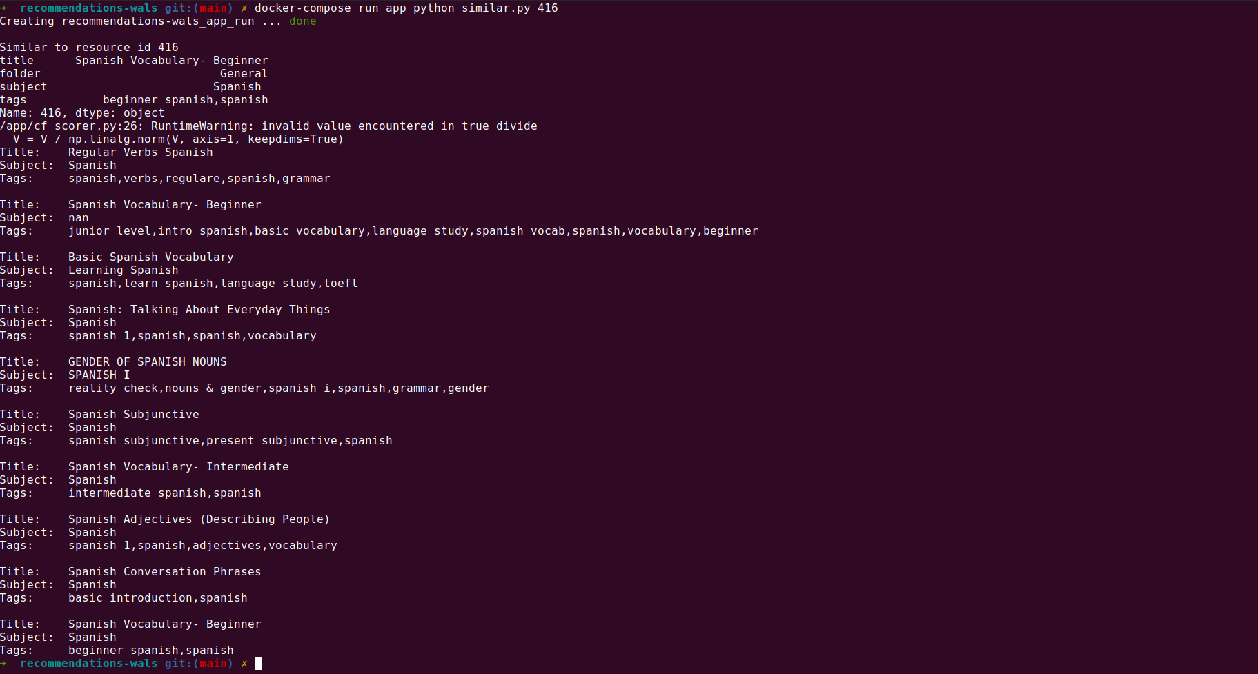
NB The ideas demonstrated for finding similar content can be used to find recommended content for a particular user. Instead of calling the
top_n method with an item embedding, we instead pass the user embedding for the user of interest.
Conclusion
Wow, this has been a long post! We have introduced the basic principles of collaborative filtering and explained the specific technique of matrix factorization. We have explained how this matrix factorization can be formulated as an optimization problem, and explained how the model can be altered to take better account of implicit feedback data.
We use the implicit library to solve the matrix factorization problem, and we have
provided code samples to outline how we can extract, filter and transform the GoConqr dataset to integrate with the implicit solver.
Finally we looked at how this model can be used to generate similar/recommended content for a given piece of content.
Whilst it feels like we covered a lot in this post, there were a few areas that we completely glossed over. These areas include the task of measuring the effectiveness of the model. This is essential to allow us to choose optimum values for our hyperparameters such as $\lambda$, $\alpha$ and $f$. I would like to revisit this in a bit more depth in a separate blog post. Also, there is the question of how we can deploy this model to make is accessible to our other applications and systems that may wish to leverage this recommendation power. Again, this particular topic will have to wait to another day. If you would like to be informed when I have released these follow up blog posts, please consider subscribing to the mailing list.
References
- Seminal paper on collaborative filtering for implicit feedback datasets from Hu, Koren & Volinsky
- Great Python Notebook from Jesse Steinweg-Woods demonstrating the ALS method for implicit data
- The implicit library from Ben Frederickson
- Blog post on music recommendations from Ben Frederickson
- The seminal Funk post about the SVD technique
- Ethan Rosenthal blog post on MF for explict datasets
- Ethan Rosenthal blog post on MF for implicit datasets
Comments
There are no existing comments
Got your own view or feedback? Share it with us below …